How To Draw An Arrow In Python

Arrows in Python Plots

An introduction to arrows and text annotations in matplotlib plots

Photograph by kaleb tapp on Unsplash

Unfortunately (or rather, fortunately), information scientific discipline has evolved to go much more than just building ML models. Harvard Business Review recently published an article¹ on what leading Data Scientists do. Surprisingly enough, the key skill is communication, rather than experience with statistical models.

If you are a data scientist, you would have known by at present t hat storytelling is your bread and butter. Every pair of stakeholders' eyes are focused on how well can you sell the story. You get a brusque window of their attending, and if you lose that window, you lose the opportunity. Believe me, it is not easy to impress the audition, specially if y'all are from a reckoner scientific discipline background. But the good part is that the art of storytelling can be learned gradually.

Maybe stories are simply data with a soul. — Brené Brown

If y'all want to be adept at communicating your analysis with the audience, then the showtime step is to larn how to present your data as visually as possible. Recent studies have plant that a picture tin get far longer than a bunch of verbose text.

The greatest value of a picture is when it forces the states to discover what we never expected to run into. -John Tukey

Methods as simple every bit annotating the graphs can do wonders. This article tries to take a stab at introducing arrows and text annotations in a plot. So, without further ado, permit's larn.

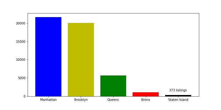
The below code reads the 2022 NYC listings² and prints the neighborhoods along with their respective count of listings institute in the dataset.

          # Read data
df = pd.read_csv('/kaggle/input/new-york-city-airbnb-open-data/AB_NYC_2019.csv')          # Get the count of the listings by neighbourhood.
nbr_freq = df.neighbourhood_group.value_counts()
impress(nbr_freq)        

Nosotros can conclude that Manhattan has a maximum number of listings (21661) while Staten Island has the to the lowest degree number of listings (373).

          Manhattan        21661
Brooklyn         20224
Queens            5666
Bronx             1091
Staten Island      373
Name: neighbourhood_group, dtype: int64        

Let's expect at how nosotros can annotate the bar respective to Staten Island with the number of listings in Staten Island. We have used annotate part to add text to the graph. The params used in the part are:

• xy — The XY coordinate of the bespeak (in the plot) to annotate
• xycoords — The coordinate system for the xy param
• horizontalalignment — The horizontal alignment of text for xy location.

Currently, we have set xycoords to information. What it means is that xy will use the axes of information as its coordinate system. Thus, in this case, x is set to Staten Island and y to 2000. You can learn most other coordinate systems here.

          import matplotlib.pyplot as plt
import random          # Define effigy size
plt.effigy(figsize=(10,5))          # Random colors for each plot bar
my_colors = ['r', 'g', 'b', 'chiliad', 'y'] #ruddy, greenish, blueish, black, etc.
random.shuffle(my_colors)          # Plot the histogram
plt.bar(nbr_freq.alphabetize, nbr_freq.values, color=my_colors)          # Get electric current axis
ax = plt.gcf().gca()          ax.comment('373 listings', xy=("Staten Island", 2000),
                        verticalalignment            ='top',             horizontalalignment            ='eye')        

Image by Author

Adding a simple arrow

At present that we sympathise how tin we place a text in a plot, permit's add together more gimmicks to it. We can add shapes (such as arrows) to the plot to make it even more appealing. The following script adds three new params to achieve this.

• xytext — The XY coordinates to place the text at.
• textcoords — The coordinate system for xytext
• arrowprops — The backdrop (dict) used to draw an arrow betwixt xy and xytext

For the beneath plot, the textcoords is set to axes fraction. Information technology ways that the location of xytext is the fraction of the axes from the lower left of the plot. You can read about different coordinate systems for textcoords here. The xytext tuple value (0.94, 0.viii) places the text by calculating the fraction of the axis in both directions. `

arrowprops dict contains numerous predefined keys to create customized shapes of the arrow. One such fundamental used here is shrinkwhich defines the fraction of the arrow length to shrink from both ends.

          ax.comment('Lowest listings',            
            xy=("Staten Island", 1000),
            xycoords='data',
            xytext=(0.94, 0.viii),            
            textcoords='axes fraction',
            arrowprops=dict(facecolor='black', shrink=0.05),
            horizontalalignment='right',
            verticalalignment='top')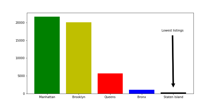        

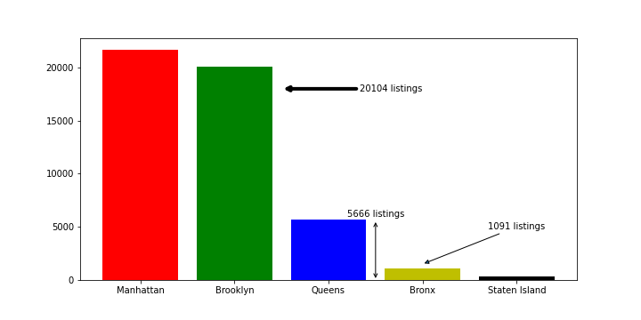
Image by Author

Calculation a fancy pointer

Using FancyArrowPatch — If yous need to add a more than sophisticated arrow, so yous need to use FancyArrowPatch . To use FancyArrowPatch you must define the arrowstyle fundamental in the arrowprops dictionary. The arrowstylefundamental determines the shape of the arrow. In that location are other central values that you tin can add together to customize the color and width of the arrow. lw is one such instance that is used to conform the arrow width. You tin explore more options in the official documentation.

          ax.annotate('1091 listings',
            xy=("Bronx", 1500),
            xytext=("Staten Island", 5000),            
            va='center',
            ha='middle',
            arrowprops={'arrowstyle': '-|>'})          ax.comment('20104 listings',
            xy=(i.5, 18000),
            xytext=("Bronx", 18000),            
            va='middle',
            ha='correct',
            arrowprops={'arrowstyle': '-|>', 'lw': iv})          ax.annotate('5666 listings',
            xy=(2.5, 0),
            xytext=(2.5, 6200),
            va='eye',
            ha='centre',
            arrowprops={'arrowstyle': '<->'})        

Image by Writer

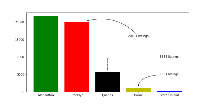
Defining ConnectionStyle

We can command the shape of the pointer by definingConnectionStyle param in arrowprops. The connectionstyle can be either of the three angle/angle3, arc, or bar. In the offset of the three examples illustrated beneath, the connectionstyle is angle3. In simple words, angle3 is used to create a elementary quadratic Bezier Curve between xy and xytext. The start and endpoints have a slope of angleA and angleB respectively. Another interesting connection style is an arc, which is used in the third case below. You tin play with different conntectionStyle here.

          # angleA = 0            
# angleB = 90
ax.comment('1091 listings', xy=("Bronx", 1500),
            xytext=("Staten Isle", 5000),            
            va='heart',            
            ha='heart',
            arrowprops={'arrowstyle': '-|>', 'connectionstyle': 'angle3,angleA=0,angleB=xc'})          # angleA = 0            
# angleB = 90
# rad = 5
ax.annotate('5666 listings', xy=("Queens", 6000),
            xytext=("Staten Island", 10000),            
            va='center',            
            ha='center',
            arrowprops={'arrowstyle': '->', 'ls':'dashed', 'connectionstyle': 'bending,angleA=0,angleB=90,rad=5'})          # angleA = 0            
# angleB = 90
# rad = 0.three
ax.annotate('20104 listings', xy=(1.3, 20300),
            xytext=("Bronx", 16000),            
            va='heart',            
            ha='center',
            arrowprops={'arrowstyle': '-|>', 'connectionstyle': 'arc3,rad=0.3'})        

Image by Author

Run into! how easy it is to add arrows to the graph. I am planning to have another commodity on interactive plots soon. Stay tuned!

References
[1]: What Data Scientists Really Practise, According to 35 Data Scientists - https://hbr.org/2018/08/what-data-scientists-really-do-according-to-35-data-scientists

[2]: New York Urban center Airbnb Open Data (CCO: Public Domain) https://www.kaggle.com/dgomonov/new-york-city-airbnb-open-data

You tin can find the python scripts for the above examples hither

If yous really liked the commodity, y'all can read another 1 well-nigh Determination Trees hither. Peace!

Source: https://towardsdatascience.com/arrows-in-python-plots-51fb27d3077b

Posted by: janousekthearly.blogspot.com

Share this post